Understanding Bring a Trailer: Hammer prices
April 7, 2022
This is part of a series of articles about the online auto auction platform, Bring a Trailer. For my other posts about Bring a Trailer, click here.
This article examines hammer prices on Bring a Trailer between October 2019 and October 2021, including their distribution, change over time and correlation to overall market condition. For more background on BaT, see my introduction in part 1.
Methodology #
For a detailed discussion of my data-gathering methodology, see part 1. To briefly summarize, I used an automated scraping script written in Python to gather data from 600 randomly selected Bring a Trailer auctions closing between 10/1/2019 and 10/30/21. After collecting this data, I wrote additional scripts for data transformation, analysis and visualization. I used pandas for data transformation and exploratory analysis. I also used statsmodels for some statistical tests. The visualizations in this article were created using the plotly and seaborn packages for Python.
Results #
In this section, we will look at the distribution of hammer prices in our sample. How much are cars selling for on Bat?
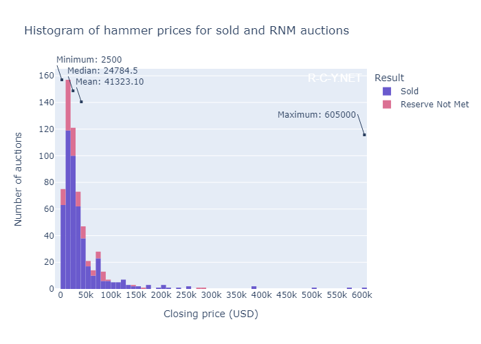
Figure 2.1: Histogram showing hammer prices for all auctions
In the above histogram, we see a right-skewed distribution for hammer prices. The prices appear to follow a log-normal distribution. Across the 600 auctions in the sample, hammer prices ranged from USD $2,500 to $605,000. The mean hammer price was $41,323.10, and the median $24,784.50. Closing prices above approx. $150k strongly skew the histogram in figure 1.1. This skewed shape indicates the prices follow a log-normal distribution.
Let’s trim the data by looking at only hammer prices within the 95th percentile. Now we can examine a histogram with more detail for the price range where 95% of auctions end.
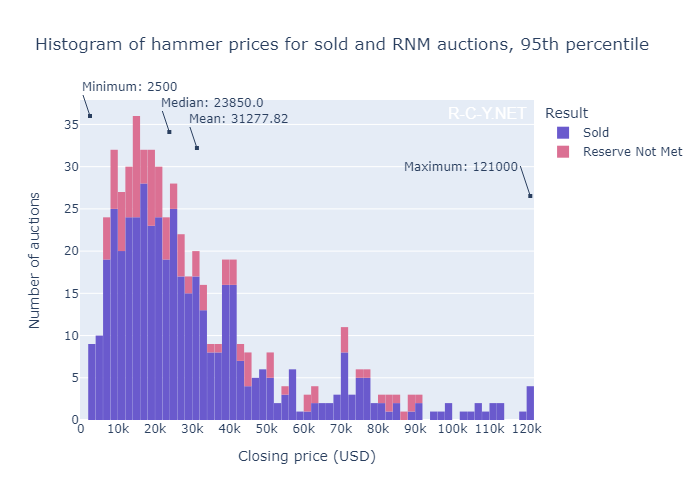
Figure 2.2: Histogram showing hammer prices within the 95th percentile
After trimming, we still see a right-skewed distribution. We see peaks in the distribution around $15k, $40k and $70k. While this gives the appearance of a multimodal distribution, a larger sample size would help demonstrate whether this is the case or if the peaks are an artifact of our sample. We can understand the overall distribution of hammer prices as the aggregate of multiple distributions of the hammer prices of individual car models. Are the peaks visible in our sample due to a tendency for hammer prices of different car models to cluster around certain mean amounts? Does this elucidate any aspect of bidder behavior, market conditions or BaT’s lot selection criteria? Evaluating these hypotheses would require a larger sample, categorized by make/model of vehicle.
When we looked at sell-through rate earlier, we compared the rate seen in the sample to that of other recent auctions. Why not do the same for the distribution of hammer prices across different auctions, in order to compare BaT to various other auction houses/platforms? An analysis by classic car insurer Hagerty shows that BaT auctions tend to bring higher prices for equivalent vehicles than sales at other venues. In the upcoming post in this series, we will look at auction results for an individual model of car. This will give us tools to develop and test hypotheses about the shape of the hammer price distributions for individual car models, how these distributions compare to the overall distribution of hammer price, and how the price distribution for certain models sold on BaT compares to other auction venues. In the meantime, let’s examine how the overall distribution of prices has changed over time.
Change over time #
As we discussed in part 1, the sample period covered by our data has seen dramatic increases in both BaT auction volume and sales totals. In the past year, BaT has also become notorious for auction results at the high end of a particular model’s market value. The Hagerty article linked above presents a data-driven argument for the existence of a “BaT premium,” which as of October 2021 they estimate is as high as 72% over the Hagerty price guide valuation for an equivalent vehicle. Their analysis also shows that this premium has increased dramatically since 2019. This dynamic is especially visible for categories of “emerging classics”, vehicles that have only recently been considered collectible or desirable by enthusiasts. BaT has achieved surprisingly high results for vehicles in this category, possibly because traditional auction houses are less inclined to accept these vehicles. Anonymous BaT commenters and respected industry publications alike take these BaT results as evidence of large-scale market shifts and revaluations.
Let’s look at some evidence of these changes. First, let’s look at a scatter plot of all hammer prices in our sample, plotted by closing time.
Note: This plot is interactive, so you can mouse over it for annotations and zoom/crop by clicking and dragging. If you have javascript disabled, you will see a non-interactive .png version.
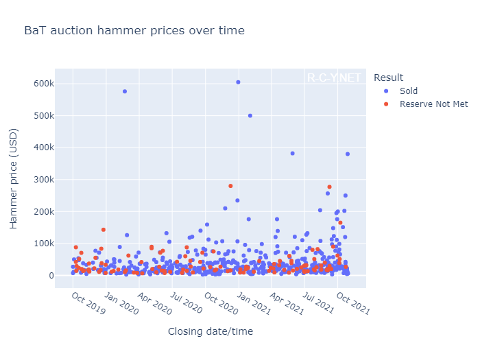
Figure 2.3: Hammer prices over time from Oct 2019-October 2021
This plot reiterates much of the information we saw in the price histogram above. Most lots end under $100k and there are a few outliers ending above $400k. There’s no dramatic changes over time, but we can see an increase in auctions closing between $100k and $200k.
Since a quick glance at the scatter plot of prices doesn’t tell us much, I performed an ordinary least squares linear regression to determine if our sample shows any statistically significant change in closing price over time. Because the prices in our sample follow a log-normal distribution, I log-transformed the prices to create a normal distribution.
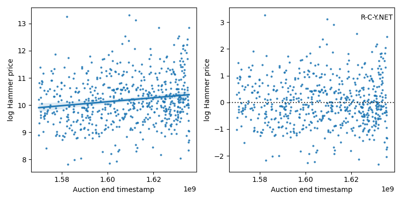
Figure 2.4: Linear regression and residual plot of log-transformed hammer prices over time
The regression line is shown on the scatter plot to the left. This regression shows a statistically significant (p=0.0001) increase over time (positive coefficient for the timestamp variable). However, the effect size is very small (R^2=0.025), meaning that increase in time only explains 2.5% of the total variation in prices across the sample. This suggests that the mean auction price on BaT has increased a small but statistically significant amount during our sample period.
The residual plot on the right shows residual values scattered at random around the horizontal axis at 0. The absence of any pattern here is a good thing, showing that our regression analysis isn’t affected by some unknown confounding variable.
How can we explain this increase in prices over time? Given the appreciation seen across the classic car market during our sample period, we can assume many models have risen in value during our sample period. Anecdotally, BaT has increased the number of “high-end” lots during the sample period, which could also drive an increase in mean hammer price. However, the small R^2 value seen in our regression indicates that an increase in prices over times only accounts for 2.5% of the observed variation in prices. This is not unexpected as BaT includes vehicles from many segments of the collector car market, each with their own price distributions and valuation trends.
BaT prices and the market #
In July 2021, Hagerty reported record growth in classic car auction sales, driven primarily by online auction sites. Given increasing total sales figures and increasing numbers of auctions on BaT, I’m curious about how closely BaT hammer prices track overall market indicators. One quantitative measure of overall market movement is the Hagerty Market Rating, a calculated index designed to track the North American collector car market.
Let’s now look at some plots comparing the overall classic car market to the hammer prices in our sample. We use the Hagerty market rating as a measure of overall market performance. This rating is calculated monthly in the middle of the month. To facilitate direct comparison between BaT hammer prices and the Hagerty rating, we will group the BaT results into groups by month, between the 15th of the named month and the previous month. For example, the October 2021 period covers September 15-October 15, approximately the same period used to calculate the October 2021 Hagerty rating.
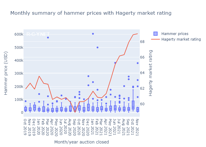
Figure 2.5: Box plots of hammer prices by month/year, with Hagerty market rating
It is difficult to determine if there is any strong correlation between BaT hammer prices and market rating using a chronological view like in Figure 1.6. An alternative approach to determine this is to calculate a Pearson correlation coefficient and associated p-value. Pearson correlation coefficients can range from -1.0 to +1.0 and represent both the direction and strength of correlation between two continuous variables. I used scipy.stats.pearsonr for this purpose, with input variables of log-transformed hammer price and the Hagerty rating for the period when each auction closed. The result was a correlation coefficient of 0.131, indicating weak positive correlation between hammer price and market rating, and a p-value of 0.001. As the p-value is below a standard significance level of 0.05, we can reject the null hypothesis that there is no correlation between hammer price and market rating. This statistical test provides evidence for a weak positive correlation between BaT hammer prices and Hagerty market rating.
While this conclusion is unsurprising given what we know about BaT’s growth and the overall market’s behavior during the last two years, it does give us data-driven evidence of a link between BaT selling prices and the overall condition of the market. However, there are some major caveats to this analysis. It’s important to understand that this correlation test does not tell us anything about the causal relationship between these two variables- we cannot state, based on this evidence alone, that the market drives BaT prices or vice versa. It’s not possible for our study to account for all the variables involved in a rigorous, experimental manner, simply because of the complexity of these kinds of market dynamics. Making causal statements puts us at risk of describing spurious relationships.
Conclusion #
- We observed a strongly right-skewed log-normal distribution of hammer prices in our sample, with a mean hammer price of approx $41k and a maximum of $605k.
- We have also plotted hammer prices over time and used linear regression to show a statistically significant increase in hammer price during our sample period.
- We also discussed the relationship between BaT prices and overall market conditions, using the Pearson correlation coefficient to show that BaT prices were positively correlated with the Hagerty market rating.
Even though there are statistically significant correlations in this data, our insight into the data remains descriptive rather than explanatory. We cannot separate out any change in prices due to BaT’s increased volume/popularity from change due to overall market movement, because these are not independent variables. Under the unique conditions created by the global pandemic, growth in the market has been supported by growth in online auction sites while traditional auction venues cancelled or shrunk their sales. This is supported by both the multiple correlations seen in our data and narratives from market experts like Hagerty. Instead of a clear explication of cause-and-effect, instead we can state that the data shows that BaT prices and wider market are coupled. While prices on BaT respond to overall market conditions, BaT’s choice of listings, increasing popularity and virality potential will also have effects on pricing across all selling venues.
In the next article in this series, I look at the effect of day of the week and weekends on auction hammer price and sell-through rate.